In the previous post I discussed my attempts at replicating a trend following algorithm. This post takes a short step back to discuss a prerequisite of running a futures trading strategy, joining the individual series together to create a continuous one.
Future instruments have an expiry date, so to trade trends that run longer than a single series you need to roll from one series to another. To simulate this in a backtest you first need to stitch them together in a fashion that replicates how you would roll when actually trading.
Rolling algorithm
The basic idea is that you roll from one future to the next at the point that the later expiring future is more liquid. There are a number of ways to determine this point, but I employed the one presented in Following the Trend, rolling when the open interest in the later future exceeds the earlier one.
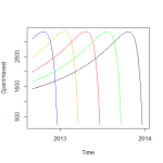
In a textbook about this you will see a graph that looks something like below. The open interest in a future steadily builds before dropping off near expiry.
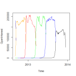
The reality might not be too far off this ideal. For example, here’s a plot of the AUD/USD open interest. There’s a very clear cut-off when the market rolls from one contract to the next.
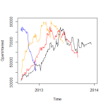
However it’s not always so clean. Here’s EuroSwiss across the same period.
As you can see it’s far less obvious. Rather than one series clearly taking over from another at one point, there are periods where the relative open interest in two series is quite closely matched. This has created situations where the rolling algorithm in the backtest doesn’t do what you would do in reality. For example, on the same EuroSwiss series there is an occasion where a series is rolled into on one day, and the very next day it is rolled out of. Each roll entails significant costs in terms of transaction fees and bid-ask spreads, so it would make no sense to do this. A more refined algorithm would be required to give a more accurate reflection of reality.
Backwardation and contango
A set of future series can either be in backwardation or contango, a description of the relative pricing levels for series on the same underlying but with different expiry dates. In the former case, futures with more distant expiry dates trade at a discount to closer expiries.
When stitching together future series the gap in prices at the roll needs to be removed to make them continuous. This has the effect of shifting historical prices either up or down, depending on whether the series is generally in backwardation or contango. A good example is natural gas.
ng = full_series_set$`Natural gas`
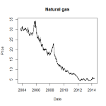
plot_series(window(ng$full_series, start=as.Date('2003-10-06'), end=as.Date('2014-05-23')), "Natural gas")
Plotting the natural gas series between 6th Oct 2003 and 23rd May 2014 gives the graph above, showing a strong downward trend. So you might expect then that the underlying spot price would have followed the same downward trajectory during this period. In fact I picked these dates because the spot price was identical at $4.40. The reason for the trend is due the roll, natural gas being in a near permanent state of contango (at least partly due to the effect of storage costs on the underlying).
I mentioned in the previous post that R can be very useful for interactive analysis of data once you’re on top of the language and the data model. Here’s a good example. What this is doing is going through all the roll details for each future series. It returns the percentage of rolls in which the more distant future, to which we are rolling, is priced lower than the current future. So a high percentage here would indicate normal backwardation, a low percentage a tendency towards contango.
data.frame(percent_backwardation = sort(round(100 * sapply(full_series_set, function (x) {
    return (nrow(x$roll_details[x$roll_details$crossover_gap < 0,]) / nrow(x$roll_details))
}), 1)))
It gives the following results.
               percent_backwardation
Gold                             0.6
DAX                              1.5
Silver                           1.7
JPY/USD                          6.9
Rough rice                      11.0
CHF/USD                         11.7
Wheat                           13.4
Natural gas                     15.5
Corn                            17.2
Nikkei 225                      23.7
Cotton                          26.4
Soybeans                        26.4
Platinum                        26.4
Palladium                       27.1
S&P 500                         27.1
Nasdaq 100                      29.0
Oats                            30.6
Lumber                          31.2
FTSE 100                        31.4
Copper                          32.3
Heating oil                     34.7
Gasoil                          36.5
CAC Index                       40.4
Live cattle                     40.6
EUR/USD                         42.0
CrudeOil                        47.2
Euribor                         49.2
Lean hogs                       50.6
Short sterling                  52.9
EuroSwiss                       57.0
Hang Seng                       58.3
EuroDollar                      66.7
CAD/USD                         68.1
Schatz                          70.8
Long gilt                       74.3
Bund                            78.5
US 2-year                       81.1
GBP/USD                         81.9
AUD/USD                         85.5
US 10-year                      88.0
NZD/USD                         98.0
This is sort of as you’d expect for the most part. The storage costs associated with commodities mean they veer towards contango. In my series there was only one backwardation roll for gold, in August 2015, which ties in with reports in the press. DAX is an interesting one. This is quoted as a performance equity index, differing from other widely used equity indexes in that dividends are included. This removes the ex-dividend effect that would otherwise affect future spot price expectations.
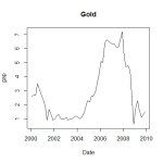
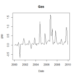
However I was expecting natural gas to be nearer the top of this list. One reason it isn’t is probably due to the seasonal behaviour. So although on average it is heavily in contango, the seasonal effect on demand for the underlying affects the forward curve and hence creates periods of backwardation in the first two futures. If I plot the gaps between adjoining futures over time you can see how gold follows a relatively smooth path, but gas does exhibit a seasonal quality.
Data quality
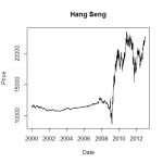
By chance I happened plot the Hang Seng series that I had just constructed from the corresponding sequence of futures. The graph is as below.
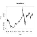
This looked very odd, surely volatility hadn’t increased that much since 2008? Indeed it had not. What had happened is that the scaling of the price changed in 2008, so that prices after that are reported as being 10 times those before. Since I was stitching them together, and removing any gaps at the roll, it gave the impression of being a continuous price series with a jump in volatility. The fix was a rather unsatisfying hack of selective rescaling, giving a more plausible looking graph below.
Conclusion
Before a backtest can be performed the basic future pricing data needs to be prepared. I was doing this by taking the free data from Quandl and stitching it together myself, but they also have a paid-for option where the data is cleaned and the roll performed in a variety of ways. I can now see the value in this. There will certainly be issues with my pricing data that I’ve not uncovered, and cases where my rolling algorithm doesn’t do the sensible thing.

